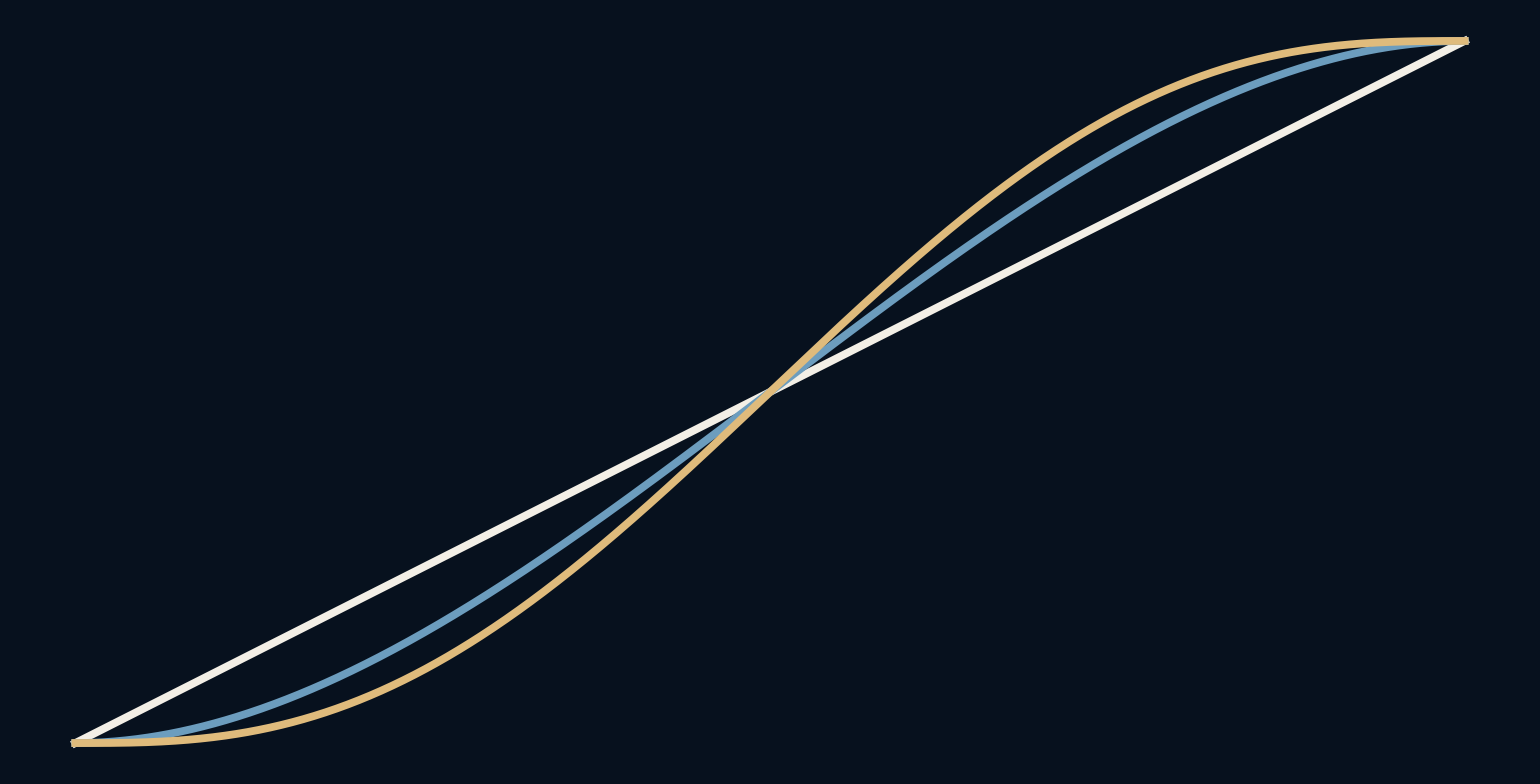
If two objects start and finish together, why can their movements look so different?
One object moves at a steady speed, another gently leaves rest and slows before arriving. Both cover the same distance in the same time. Their difference is contained in how progress is distributed between the endpoints. Three simple curves expose that choice, along with a less obvious consequence: gentler departures require faster movement somewhere in the middle.
A gentle start borrows speed from the middle.
Progress is a function, not a frame count
Let u run from zero to one over the animation's duration. A progress function maps u to the fraction of the distance travelled. Linear interpolation uses u itself, so equal time intervals cover equal distances. It is predictable and easy to synchronize with another steadily changing quantity.
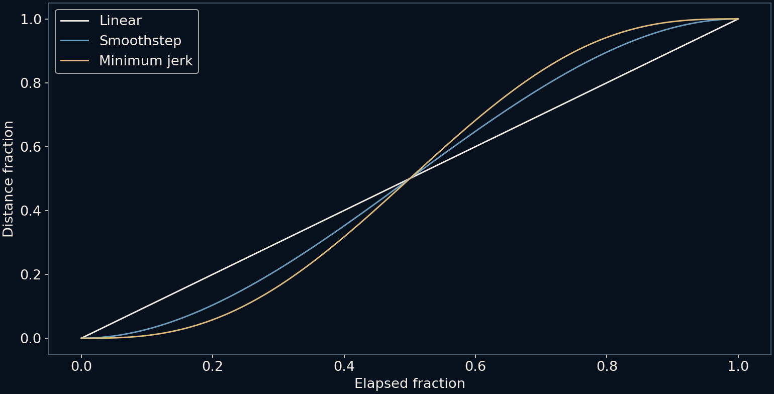
Our comparison uses one distance unit and one second, keeping the units explicit. All three curves start at position zero and finish at one. None overshoots. The question is not which reaches the destination first, but what its position, speed and acceleration are while making the same scheduled journey.
A useful implementation distinction follows from normalized time. Evaluate progress from elapsed time divided by the intended duration, rather than adding a fixed amount whenever a frame happens to render. If a frame is late, the next sample can still represent the scheduled moment. That preserves the timing relationship, although it may produce a visible jump across the missed positions. A correct clock does not guarantee that every intermediate image was displayed.
Smoothstep changes the departure
The cubic smoothstep curve is three times u squared minus two times u cubed. Its slope is zero at both ends, so it can join a stationary position without an instantaneous jump in speed. The curve rises more slowly at first, moves faster around halfway and then slows again.
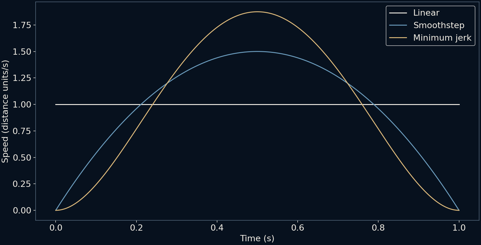
Its maximum speed is 1.5 distance units per second in this example, compared with one for linear motion. That increase is unavoidable for some part of any journey that spends extra time moving slowly but must retain the same total distance and duration. Smooth-looking motion does not necessarily mean low peak speed.
A fifth-degree curve smooths another boundary
The minimum-jerk progress curve used here is 10u cubed minus 15u to the fourth plus 6u to the fifth. It has zero velocity and zero acceleration at both endpoints. Its peak speed is 1.875 units per second, higher than the cubic's, because it devotes more of the interval to its gentle entry and exit.
Jerk is the rate of change of acceleration. Under fixed endpoints, duration, and zero endpoint velocity and acceleration, this polynomial minimizes the integral of squared jerk for the one-dimensional motion. That precise mathematical property gives the curve its name. It does not establish that every interface animation should use it or that all human movement follows it.
Minimum jerk does not mean zero jerk everywhere. Differentiating the fifth-degree curve a third time gives 60 − 360u + 360u² in normalized units. At both endpoints its value is 60, whereas an object held at rest outside the interval has zero jerk. The position, velocity and acceleration can join continuously while jerk still jumps. The minimized quantity is an integral over the journey, not a promise that every instantaneous derivative is the smallest possible.
Look at derivatives, not only the pretty curve
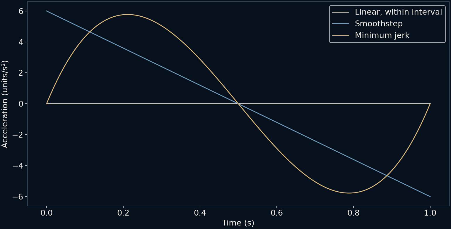
The position plots all look orderly. The speed plot reveals their different peaks, and the acceleration plot reveals different endpoint behaviour. Within its interval, linear motion has zero acceleration, but joining it to rest requires an abrupt speed change at the start and finish. Those boundary impulses are not drawn as finite values in the plot.
Smoothstep reaches the endpoints with acceleration of plus six and minus six units per second squared. If the object is stationary outside the interval, acceleration therefore jumps at the joins. The fifth-degree curve meets zero acceleration smoothly, though higher derivatives still have their own boundary behaviour. Smoothness always needs a stated order and a stated joining condition.
Duration changes the physical demands
The graphs are normalized examples, not a fixed recipe for every distance. Scaling the distance by D and the duration by T scales velocity by D divided by T and acceleration by D divided by T squared. Halving the duration doubles the speed and quadruples the acceleration for the same path and curve.
This matters in physical motion control, where limits cannot be judged from an attractive easing shape alone. It also matters visually: a curve that feels calm over a long transition can look abrupt when squeezed into a short one. Frame cadence and display response add further constraints that our continuous equations do not simulate.
Give the example a screen-sized scale: travel 300 pixels in 0.6 seconds. The continuous peak speeds become 500 pixels per second for linear motion, 750 for smoothstep and 937.5 for minimum jerk. The latter two peak acceleration magnitudes are approximately 5,000 and 4,811 pixels per second squared, respectively. Their ordering differs from the peak-speed ordering. Those are demands of the specified curves, not measurements of a display or a recommendation for a physical actuator.
Choose motion for what it needs to communicate
Constant speed can be appropriate for a moving timeline or a process intended to appear steady. A gentle settle may help an object look as though it arrives and stops. Overshoot, bounce and other styles require different rules, and their usefulness depends on context rather than on a universal hierarchy from mechanical to natural.
The calculation offers a vocabulary for those choices without claiming a user-perception experiment. Inspect position to see where the object is, speed to see how quickly it travels and acceleration to see how the speed changes. Once these are separated, easing becomes a deliberate allocation of motion rather than a decorative preset chosen by name.
What a finite sequence actually samples
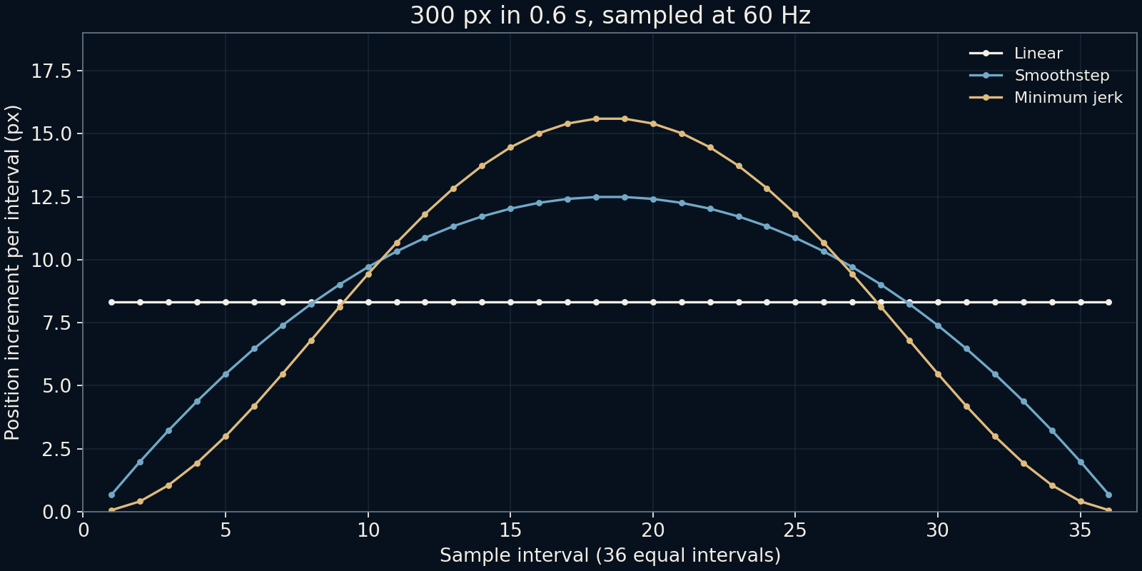
Sample that 300-pixel journey at exactly 60 equally spaced instants per second. The 0.6-second interval contains 36 steps and 37 endpoint-inclusive positions. Linear motion advances about 8.333 pixels per step. The first smoothstep increment is only 0.682 pixels, and the first minimum-jerk increment is about 0.062 pixels. Fractional positions are meaningful in this calculation, even though a particular renderer may represent or round them differently.
The middle of the journey makes up that early difference. The largest sampled increments are approximately 12.487 pixels for smoothstep and 15.593 for minimum jerk. These finite differences are average travel over an interval, rather than the continuous velocity at one exact instant. The new figure plots all 36 increments so the gentle ends and expensive middle can be inspected together. It also shows why counting only the total frames misses an important part of the motion.
By 100 milliseconds, the three curves have covered 50.000, 22.222 and 10.648 pixels, in the same order. A very gentle start can therefore delay visible progress, even when the final arrival time is unchanged. For a control that should acknowledge an action quickly, consider that early trajectory as well as the settling motion. For physical movement, check velocity, acceleration, jerk and the actual mechanism separately. This calculation exposes trade-offs without assigning one curve a universal claim to responsiveness or comfort.
Further reading
Khronos: GLSL smoothstep ↗Flash and Hogan: The coordination of arm movements ↗MDN: CSS easing functions ↗Original documentation and useful background.