
Six out of ten and six hundred out of a thousand are both 60%.
Imagine an imaginary coin-like choice that succeeds with a fixed probability of 0.6. The experiment knows that probability because it creates the world. An observer sees only successes and attempts. A sample of ten can look very different from the next sample of ten. Larger independent samples tend to concentrate more tightly, even though their displayed percentage may look just as simple.
The denominator is part of the evidence.
Sixty percent leaves something unsaid
Six successes in ten attempts produce exactly the same fraction as 600 in 1,000. The arithmetic has erased the sample size. But one changed outcome moves the first estimate by ten percentage points and the second by only one tenth of a point. Equal fractions therefore need not carry equal precision.
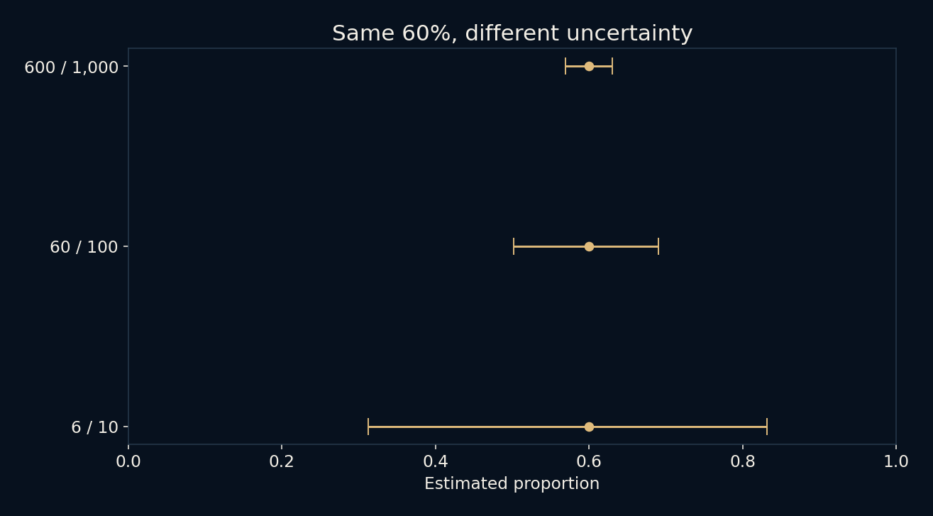
The experiment compares 6/10, 60/100 and 600/1,000 using a 95% Wilson interval. This method adjusts both the centre and width rather than placing a simple symmetric band around every observed fraction. It behaves sensibly near zero and one, where an unrestricted approximation could wander outside the possible probability range.
A wider interval is a useful admission
For 6/10, the computed interval runs from about 31.27% to 83.18%. For 60/100, it is 50.20% to 69.06%. For 600/1,000, it is 56.93% to 62.99%. All three observations say 60%, but the ranges make their very different precision visible without inventing extra decimal places.
These intervals refer to a procedure under an independent binary-trial model. In the usual frequentist interpretation, the fixed unknown proportion is not assigned a 95% probability of being inside this particular realized interval. Instead, the method aims for approximately 95% coverage over repeated samples. That distinction is easy to lose when a chart looks like a probability cloud.
Watch many new samples
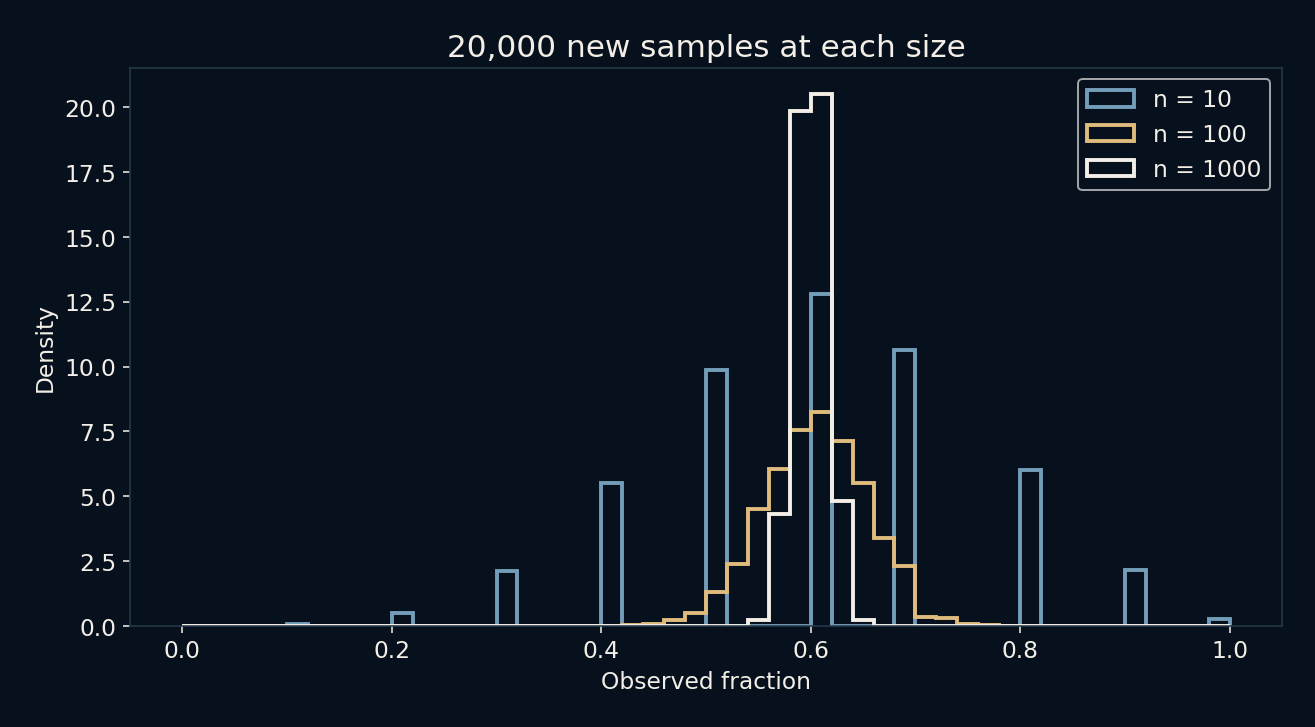
The script generated 20,000 independent samples at each of the three sizes, always using the true success probability 0.6. Their observed fractions spread widely at ten attempts and gather more closely around 0.6 at a thousand. The histogram shows this repeated-sampling behaviour, rather than suggesting that one observed sample contains many possible realities.
It also checked how often each computed interval covered 0.6. The measured coverages were 98.33%, 94.73% and 95.16% for sizes 10, 100 and 1,000. A method labeled 95% need not achieve exactly 95% at every sample size and underlying probability. Binary counts live on a discrete grid, and the simulation itself has finite sampling variation.
Four times as many is not four times as precise
For independent binary observations away from the boundaries, the familiar standard-error scale is proportional to one over the square root of sample size. Roughly halving that kind of uncertainty therefore requires about four times as many observations, not twice as many. The Wilson formula contains further finite-sample adjustments.
This square-root relationship explains why adding a few more responses to a tiny sample can matter, while shaving a little uncertainty off an already large study can be expensive. It is a model-based relationship, not a promise that each new response moves an estimate toward the truth. A longer individual sequence can temporarily move farther away.
More of the wrong sample is still the wrong sample
The experiment grants independence and a constant probability by construction. Real polls or measurements may overrepresent a group, repeat the same person, miss nonresponders or change their question halfway through. A narrow interval from the wrong sampling model can be very confident about a biased answer. Sample size alone cannot repair that.
Before trusting an impressive denominator, ask how observations were selected and whether they bring genuinely new information. Then choose an interval suited to the design and the decision. The small sample is not worthless; it is simply less precise under this model. Showing its uncertainty is more informative than pretending its neat percentage says everything.
Further reading
NIST: confidence limits for a proportion ↗NumPy: binomial sampling ↗Original documentation and useful background.